Ridge Regression
Math 158 - Spring 2022
Jo Hardin (from Julia Silge)
Data & goal
- dataset is from TidyTuesday.
- we explore the information from The Office.
- analysis taken from Julia Silge’s blog.
- she does a bit of data wrangling that I’m going to hide. Look through her blog, or see the source code for this bookdown file.
Modeling prep
Split data into training and testing
set.seed(47)
office_split <- initial_split(office, strata = season)
office_train <- training(office_split)
office_test <- testing(office_split)

office
# A tibble: 136 × 32
season episode episode_name andy angela darryl dwight jim kelly kevin
<dbl> <dbl> <chr> <int> <int> <int> <int> <int> <int> <int>
1 1 1 pilot 0 1 0 29 36 0 1
2 1 2 diversity day 0 4 0 17 25 2 8
3 1 3 health care 0 5 0 62 42 0 6
4 1 5 basketball 0 3 15 25 21 0 1
5 1 6 hot girl 0 3 0 28 55 0 5
6 2 1 dundies 0 1 1 32 32 7 1
7 2 2 sexual harassment 0 2 9 11 16 0 6
8 2 3 office olympics 0 6 0 55 55 0 9
9 2 4 fire 0 17 0 65 51 4 5
10 2 5 halloween 0 13 0 33 30 3 2
# … with 126 more rows, and 22 more variables: michael <int>, oscar <int>,
# pam <int>, phyllis <int>, ryan <int>, toby <int>, erin <int>, jan <int>,
# ken_kwapis <dbl>, greg_daniels <dbl>, b_j_novak <dbl>,
# paul_lieberstein <dbl>, mindy_kaling <dbl>, paul_feig <dbl>,
# gene_stupnitsky <dbl>, lee_eisenberg <dbl>, jennifer_celotta <dbl>,
# randall_einhorn <dbl>, brent_forrester <dbl>, jeffrey_blitz <dbl>,
# justin_spitzer <dbl>, imdb_rating <dbl>Full linear model
office_lm <- office_train %>%
  select(-episode_name) %>%
  lm(imdb_rating ~ ., data = .)

office_lm %>% tidy()
# A tibble: 31 × 5
term estimate std.error statistic p.value
<chr> <dbl> <dbl> <dbl> <dbl>
1 (Intercept) 7.19 0.315 22.8 3.83e-34
2 season -0.00222 0.0366 -0.0607 9.52e- 1
3 episode 0.0145 0.00730 1.98 5.15e- 2
4 andy 0.00215 0.00424 0.507 6.14e- 1
5 angela 0.00307 0.00865 0.354 7.24e- 1
6 darryl 0.000932 0.00783 0.119 9.06e- 1
7 dwight -0.00172 0.00380 -0.452 6.53e- 1
8 jim 0.00541 0.00375 1.44 1.54e- 1
9 kelly -0.0129 0.0101 -1.28 2.05e- 1
10 kevin 0.00279 0.0114 0.244 8.08e- 1
# … with 21 more rowsWhat if \(n\) is really small?
set.seed(47)
office_train %>%
  select(-episode_name) %>%
  slice_sample(n = 5) %>%
  lm(imdb_rating ~ ., data = .) %>%
  tidy()
# A tibble: 31 × 5
term estimate std.error statistic p.value
<chr> <dbl> <dbl> <dbl> <dbl>
1 (Intercept) 7.30 NaN NaN NaN
2 season 0.228 NaN NaN NaN
3 episode 0.0264 NaN NaN NaN
4 andy -0.0197 NaN NaN NaN
5 angela 0.0499 NaN NaN NaN
6 darryl NA NA NA NA
7 dwight NA NA NA NA
8 jim NA NA NA NA
9 kelly NA NA NA NA
10 kevin NA NA NA NA
# … with 21 more rowsCreate recipe
Create workflow
mixture = 0 means ridge regression (mixture = 1 means Lasso)
Ridge Regression Output
# A tibble: 31 × 3
   term         estimate penalty
   <chr>           <dbl>   <dbl>
 1 (Intercept)  8.36          47
 2 season      -0.00110       47
 3 episode      0.00107       47
 4 andy        -0.000546      47
 5 angela       0.00106       47
 6 darryl       0.000434      47
 7 dwight       0.000952      47
 8 jim          0.00150       47
 9 kelly        0.000112      47
10 kevin        0.000600      47
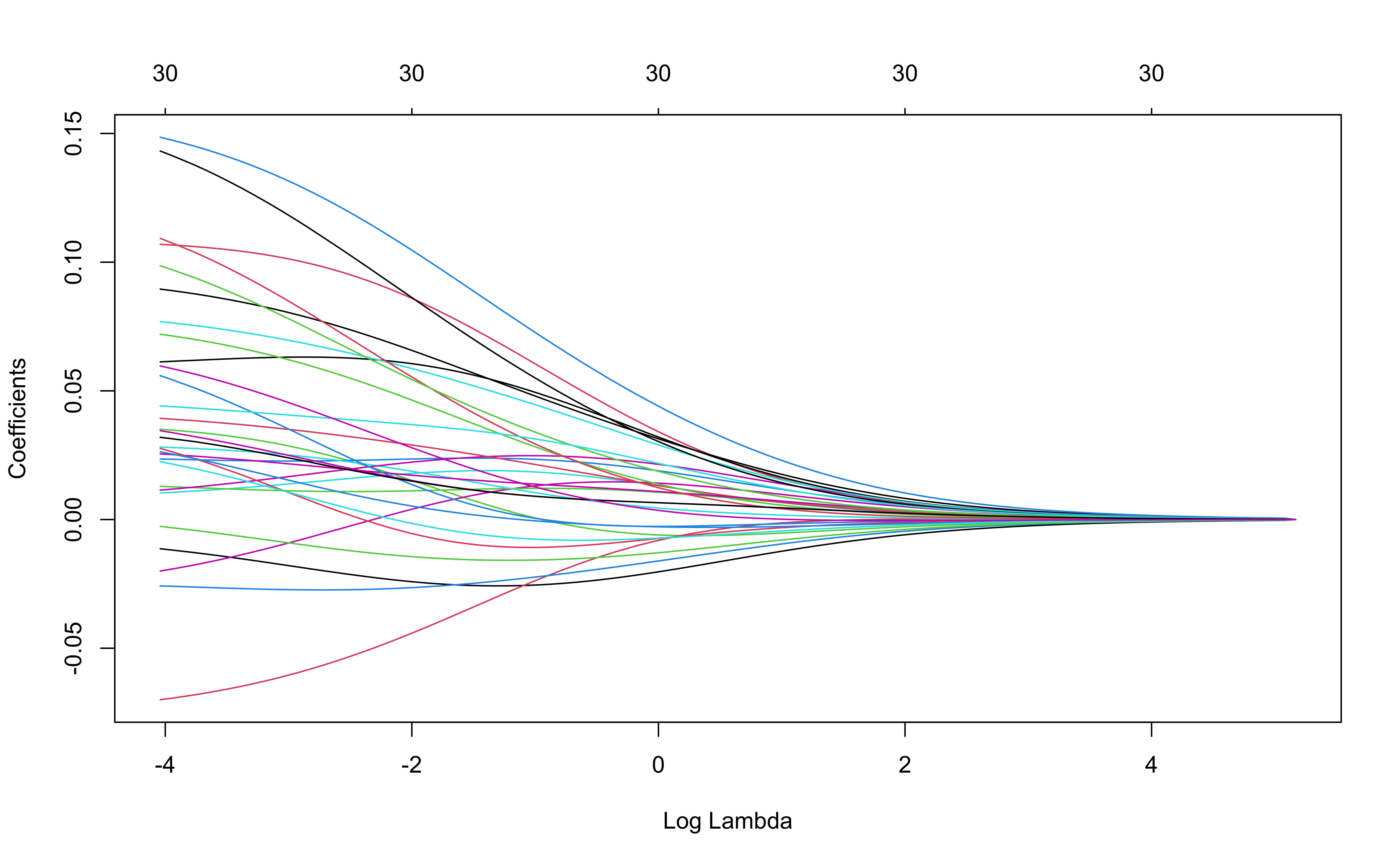
# … with 21 more rowsCoefficients as a function of lambda

How do we find lambda?
We tune() (instead of setting the penalty)
New workflow with tuned engine
ridge_spec_tune was created with tune()
set.seed(1234)
office_fold <- vfold_cv(office_train, strata = season)

ridge_grid <- grid_regular(penalty(range = c(-5, 5)), levels = 50)

ridge_wf <- workflow() %>%
  add_recipe(office_rec)

ridge_fit <- ridge_wf %>%
  add_model(ridge_spec_tune) %>%
  fit(data = office_train)

# this is the line that tunes the model using cross validation
set.seed(2020)
ridge_cv <- tune_grid(
  ridge_wf %>% add_model(ridge_spec_tune),
  resamples = office_fold,
  grid = ridge_grid
)
Which lambda is best?
# A tibble: 50 × 7
   penalty .metric .estimator  mean     n std_err .config
     <dbl> <chr>   <chr>      <dbl> <int>   <dbl> <chr>
 1   0.791 rmse    standard   0.465    10  0.0369 Preprocessor1_Model25
 2   0.494 rmse    standard   0.466    10  0.0385 Preprocessor1_Model24
 3   1.26  rmse    standard   0.467    10  0.0357 Preprocessor1_Model26
 4   0.309 rmse    standard   0.470    10  0.0406 Preprocessor1_Model23
 5   2.02  rmse    standard   0.472    10  0.0349 Preprocessor1_Model27
 6   0.193 rmse    standard   0.476    10  0.0427 Preprocessor1_Model22
 7   3.24  rmse    standard   0.477    10  0.0344 Preprocessor1_Model28
 8   5.18  rmse    standard   0.483    10  0.0341 Preprocessor1_Model29
 9   0.121 rmse    standard   0.484    10  0.0447 Preprocessor1_Model21
10   8.29  rmse    standard   0.488    10  0.0339 Preprocessor1_Model30
# … with 40 more rows
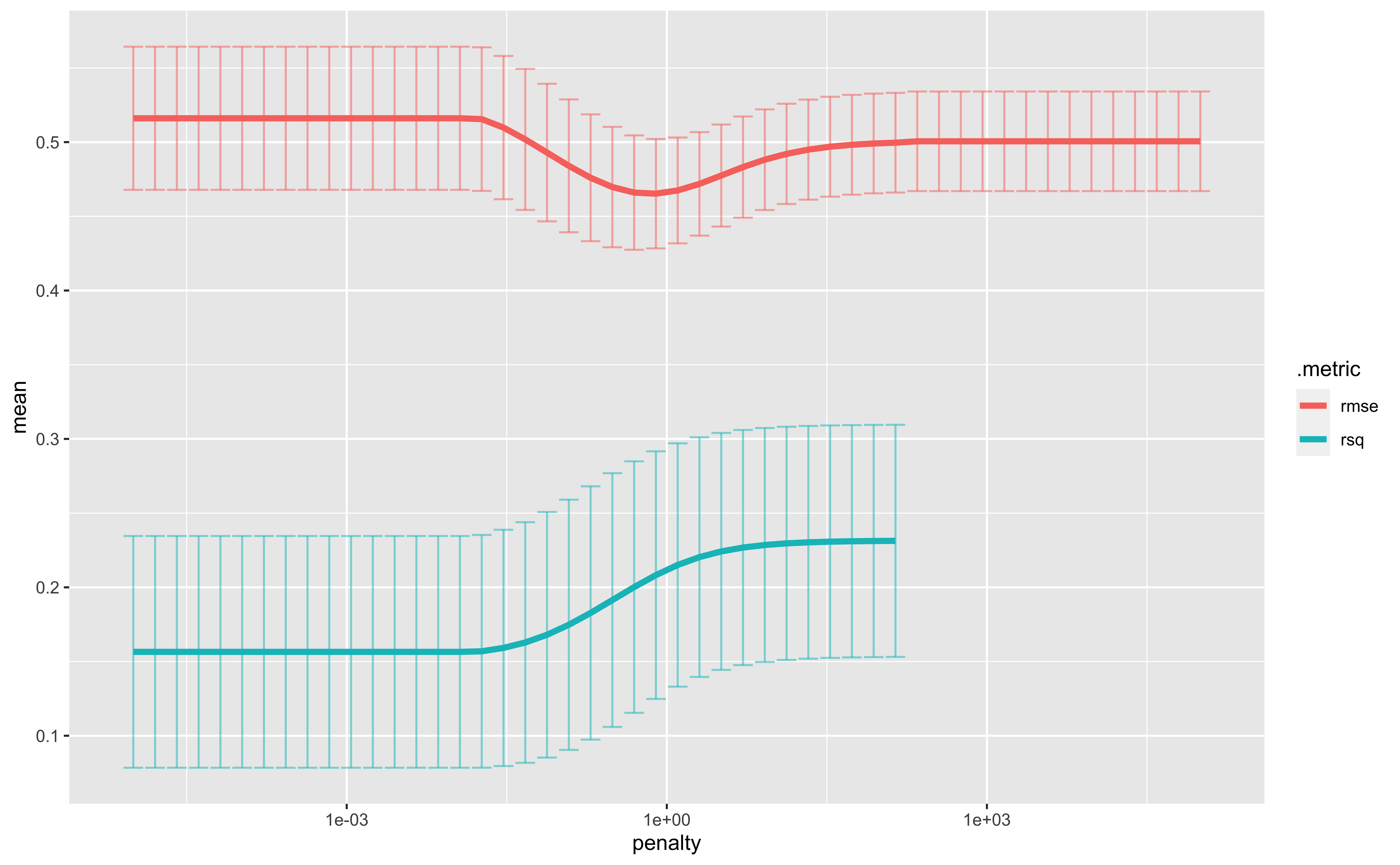
Visualizing RMSE

Best model
Final Ridge Model
finalize_workflow(ridge_wf %>% add_model(ridge_spec_tune), best_rr) %>%
  fit(data = office_test) %>% tidy()
# A tibble: 31 × 3
term estimate penalty
<chr> <dbl> <dbl>
1 (Intercept) 8.42 0.791
2 season -0.0327 0.791
3 episode 0.0383 0.791
4 andy 0.00211 0.791
5 angela 0.0233 0.791
6 darryl 0.0264 0.791
7 dwight 0.0523 0.791
8 jim 0.0407 0.791
9 kelly -0.0347 0.791
10 kevin 0.0371 0.791
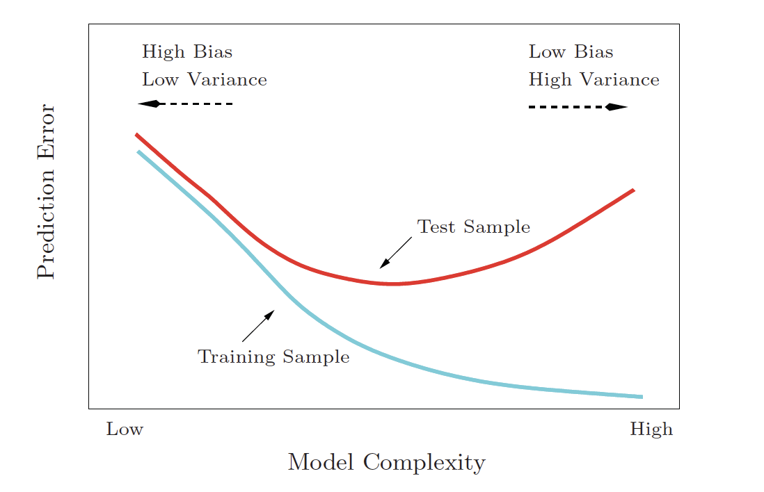
# … with 21 more rowsBias-Variance tradeoff

Credit: An Introduction to Statistical Learning, James et al.
